machine learning +
Understanding Confidence Intervals: A spelled out guide to clarify misconceptions
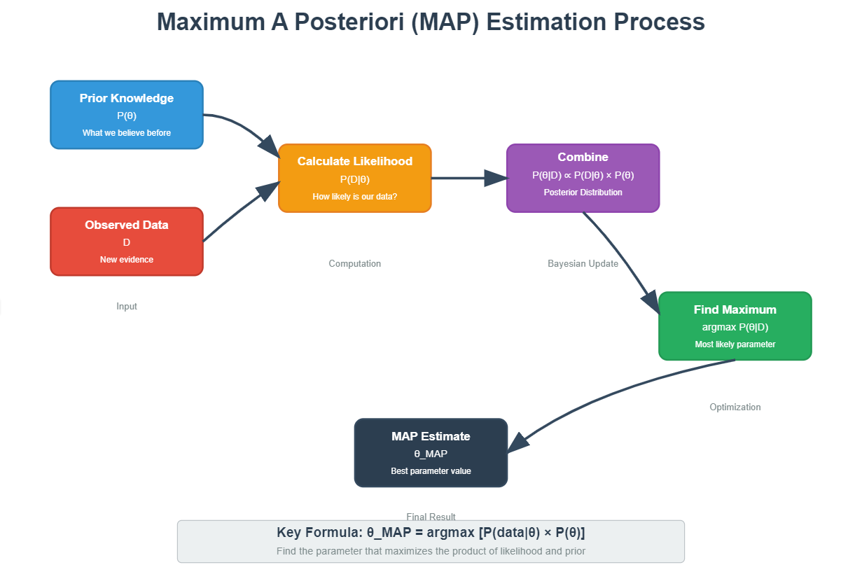
Maximum A Posteriori (MAP) Estimation – Clearly Explained
Maximum A Posteriori (MAP) estimation is a Bayesian method for finding the most likely parameter values given observed data and prior knowledge. Unlike maximum likelihood estimation which only considers the data, MAP combines what we observe with what we already know (or believe) about the parameters.
Maximum A Posteriori (MAP) estimation is a Bayesian method for finding the most likely parameter values given observed data and prior knowledge. Unlike maximum likelihood estimation which only considers the data, MAP combines what we observe with what we already know (or believe) about the parameters.
Ever wondered how your smartphone’s autocorrect gets better over time? Or how recommendation systems seem to know your preferences even with limited data? That’s the principle of MAP estimation at work – a smart way to make predictions by combining new evidence with existing knowledge.
Think of MAP as your wise friend who gives advice. They don’t just look at today’s events (the data) but also consider everything they know about you from the past (prior knowledge) to give you the best guidance.
1. The Intuition Behind MAP Estimation
Let me start with a simple story that will make everything clear.
Imagine you’re a detective investigating a crime. You have two pieces of information:
- Evidence from the crime scene (this is your data/likelihood)
- What you know about the suspect’s history (this is your prior knowledge)
A good detective doesn’t just look at today’s evidence. They combine it with background knowledge to reach the most reasonable conclusion. That’s exactly what MAP estimation does in machine learning.
MAP estimation was formally introduced in the context of Bayesian statistics, with significant contributions from Thomas Bayes (18th century) and later formalized by Pierre-Simon Laplace. The modern computational approach to MAP estimation was developed alongside the advancement of Bayesian methods in the mid-20th century.
2. The Mathematical Foundation
Here’s the core idea in one equation. Don’t let the math scare you – I’ll break it down:
python
MAP estimate = argmax P(θ|data) = argmax P(data|θ) × P(θ)
Let me translate this into plain English:
- P(data|θ), aka Likelihood: “How likely is our data given a specific parameter value?”
P(θ), aka Prior: “What did we believe about θ before seeing any data?”
P(θ|data), aka Posterior: Your updated belief after seeing the data, which is, “What’s the probability of our parameter θ given the data we observed?”
MAP estimation is based on Bayes’ theorem, which you can think of as a way to update your beliefs when you get new information:
Posterior ∝ Likelihood × Prior
MAP finds the parameter values that maximize this posterior probability. The original concept was formalized by Thomas Bayes in the 18th century and later developed into modern MAP estimation by statisticians in the 20th century.
Let’s expand on the idea a little bit more.
3. Core Idea behind MAP Estimation: (I’ll try to Keep It Simple, but skip and move to the code if this is too much)
MAP estimation is a Bayesian approach to estimate an unknown parameter (θ) by finding the value that maximizes the posterior probability distribution.
- Posterior Probability (P(θ|X)):
The probability of the parameter θ given the observed data X. Computed using Bayes’ Theorem:
$$
P(\theta|X) = \frac{P(X|\theta) \cdot P(\theta)}{P(X)}
$$
- Likelihood (P(X|θ)): Probability of data (X) given θ (from your model).
- Prior (P(θ)): Initial belief about θ (e.g., in coin toss, θ is P(head) is near 0.5).
- Evidence (P(X)): Probability of data (is constant, independent of θ).
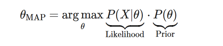
Goal of MAP:
Find the θ that maximizes the posterior probability.
$$
\theta_{\text{MAP}} = \underset{\theta}{\arg\max} \, P(\theta|X)
$$
Since $(P(X)$ in the denominator is constant, because the observed data does not change, we ignore it and maximize the numerator:
Now since the numerator contains multiplication and since the probability values are between 0 and 1, multiplying priors and likelihoods are going to give very small fractions. So, instead we take ‘log’ so that we will be able to add the values instead.
- Logarithm Trick:
Convert products to sums (easier for optimization):
$$
\theta_{\text{MAP}} = \underset{\theta}{\arg\max} \, \left[ \log P(X|\theta) + \log P(\theta) \right]
$$
- $\log P(X|\theta)$: Log-likelihood (measures data fit).
- $\log P(\theta)$: Log-prior (regularizes using prior knowledge).
- Optimize:
Solve using calculus (e.g., set derivative to zero) or numerical methods.
That’s the theory, but that doesn’t do much if we are not able to relate to a practical example. So, let’s see one and then get to the code implementations.
4. A Practical Explanation: The Cookie Jar Example
Imagine you have 2 cookie jars:
- Jar A: 70% chocolate chips, 30% raisins
- Jar B: 30% chocolate chips, 70% raisins
You randomly pick a jar (you don’t know which) and draw 3 cookies:
Chocolate, Raisin, Raisin
What jar did it come from?
- Your Prior Belief:
You think both jars are equally likely to be picked.
→ P(Jar A) = 50%, P(Jar B) = 50% The Data (Likelihood):
- Probability of drawing one chocolate and two raisins from Jar A:
0.7 (choc) × 0.3 (raisin) × 0.3 (raisin) = 0.063 - Probability from Jar B:
0.3 × 0.7 × 0.7 = 0.147
- Probability of drawing one chocolate and two raisins from Jar A:
- MAP Combines Both:
Multiply prior belief × data probability:- Jar A:
0.5 × 0.063 = 0.0315 - Jar B:
0.5 × 0.147 = 0.0735
- Jar A:
MAP picks Jar B because 0.0735 > 0.0315!
→ It’s the most probable jar given your data + prior belief.
Why Not Just Use Data Alone? (MLE vs. MAP)
- MLE (Maximum Likelihood): Only uses data.
In our example, MLE would pick Jar B too (because 0.147 > 0.063). - But if your prior changes…
Suppose you know Jar A is used 90% of the time:
P(Jar A) = 0.9,P(Jar B) = 0.1
Now:- Jar A:
0.9 × 0.063 = 0.0567 - Jar B:
0.1 × 0.147 = 0.0147
MAP picks Jar A!
→ Your strong prior belief overruled the data.
- Jar A:
In one sentence: MAP is your “best guess” after combining new evidence with what you already believed.
5. Setting Up Your Environment
Before we dive into the code, let’s get everything ready. I assume you’re comfortable with Python and have VS Code set up.
python
# !pip install numpy scipy matplotlib seaborn pandas scikit-learn jupyter
python
import numpy as np
import matplotlib.pyplot as plt
import scipy.stats as stats
from scipy.optimize import minimize_scalar
import seaborn as sns

# Set up plotting style
plt.style.use('seaborn-v0_8')
sns.set_palette("husl")
Let’s also create some helper functions we’ll use throughout:
python
def plot_distribution(x, y, title, xlabel, ylabel):
    """Helper function to create clean plots"""
    plt.figure(figsize=(10, 6))
    plt.plot(x, y, linewidth=2)
    plt.title(title, fontsize=14, fontweight='bold')
    plt.xlabel(xlabel, fontsize=12)
    plt.ylabel(ylabel, fontsize=12)
    plt.grid(True, alpha=0.3)
    plt.show()

def normalize_distribution(values):
    """Normalize values to form a probability distribution"""
    return values / np.trapz(values)
4. A Real-World Example: Estimating Coin Bias
Let’s start with something concrete. Imagine you find a coin and want to know if it’s fair. You flip it 10 times and get 7 heads.
Question: What’s your best estimate of the coin’s bias (probability of heads)?
Let me show you three different approaches and see how they compare:
python
# Our data: 10 flips, 7 heads
n_flips = 10
n_heads = 7

print(f"Observed data: {n_heads} heads out of {n_flips} flips")
print(f"That's {n_heads/n_flips:.1%} heads")
python
Observed data: 7 heads out of 10 flips
That's 70.0% heads
4.1 Maximum Likelihood Estimation (MLE)
First, let’s see what Maximum Likelihood Estimation would tell us:
python
# MLE simply uses the observed frequency
mle_estimate = n_heads / n_flips
print(f"MLE estimate: {mle_estimate:.3f} (or {mle_estimate:.1%})")
python
MLE estimate: 0.700 (or 70.0%)
MLE says: “Based purely on the data, the coin has a 70% chance of heads.”
4.2 MAP Estimation with a Fair Coin Prior
Now let’s use MAP estimation. We’ll start with a prior belief that most coins are roughly fair:
python
# Define our prior belief (Beta distribution)
# Beta(2,2) is centered at 0.5 but allows some uncertainty
prior_alpha = 2
prior_beta = 2

# After observing data, posterior is Beta(prior_alpha + heads, prior_beta + tails)
posterior_alpha = prior_alpha + n_heads
posterior_beta = prior_beta + (n_flips - n_heads)

# MAP estimate is the mode of the posterior Beta distribution
map_estimate = (posterior_alpha - 1) / (posterior_alpha + posterior_beta - 2)

print(f"MAP estimate: {map_estimate:.3f} (or {map_estimate:.1%})")
print(f"Posterior parameters: α={posterior_alpha}, β={posterior_beta}")
python
MAP estimate: 0.667 (or 66.7%)
Posterior parameters: α=9, β=5
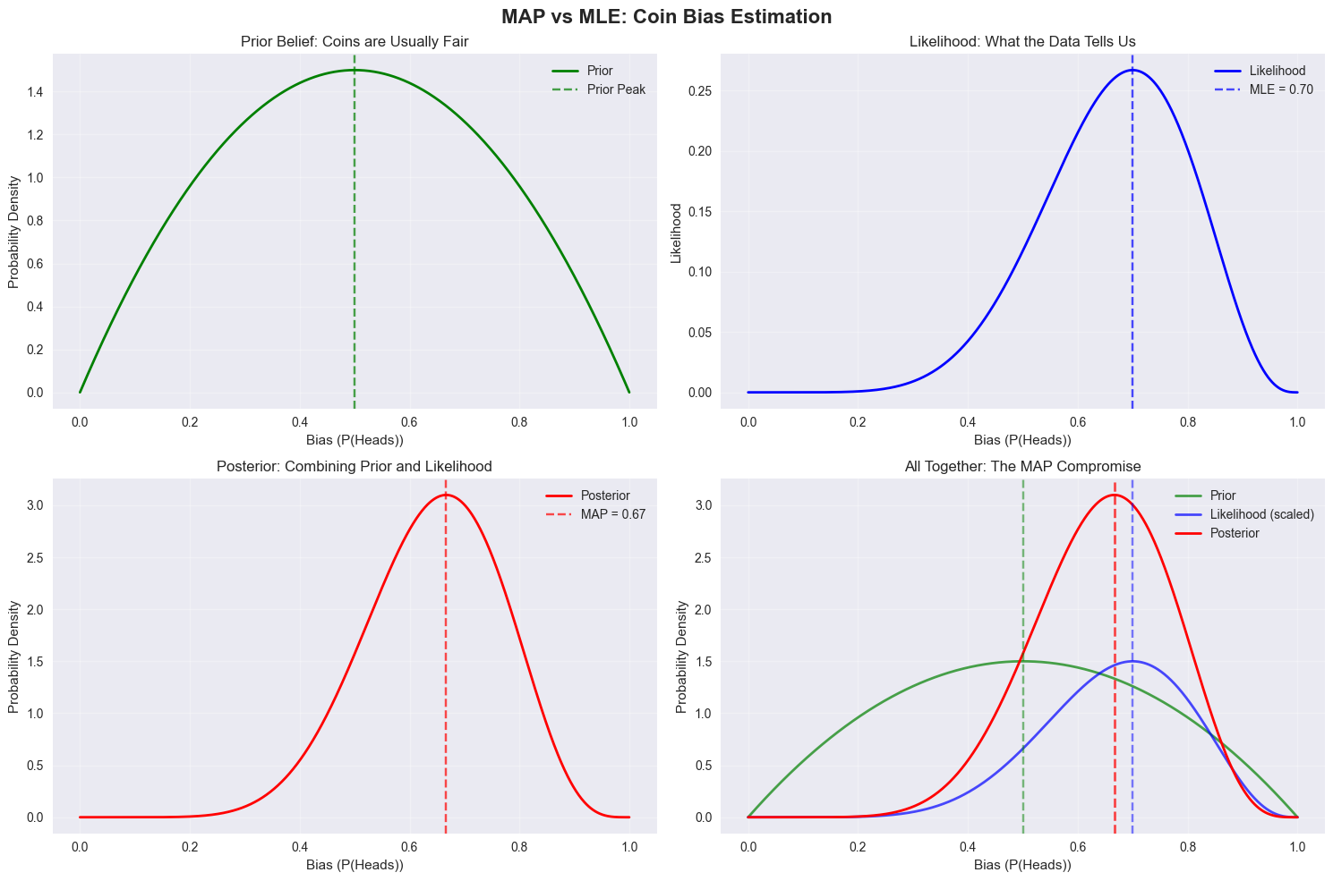
4.3 Visualizing the Difference
Let’s see this graphically to understand what’s happening:
python
# Create range of possible bias values
theta_range = np.linspace(0, 1, 1000)

# Calculate likelihood for each possible bias
likelihood = stats.binom.pmf(n_heads, n_flips, theta_range)

# Calculate prior for each possible bias
prior = stats.beta.pdf(theta_range, prior_alpha, prior_beta)

# Calculate posterior (likelihood × prior, normalized)
posterior = stats.beta.pdf(theta_range, posterior_alpha, posterior_beta)

# Create the plot
fig, axes = plt.subplots(2, 2, figsize=(15, 10))
fig.suptitle('MAP vs MLE: Coin Bias Estimation', fontsize=16, fontweight='bold')

# Plot 1: Prior belief
axes[0,0].plot(theta_range, prior, 'g-', linewidth=2, label='Prior')
axes[0,0].set_title('Prior Belief: Coins are Usually Fair')
axes[0,0].set_xlabel('Bias (P(Heads))')
axes[0,0].set_ylabel('Probability Density')
axes[0,0].axvline(0.5, color='g', linestyle='--', alpha=0.7, label='Prior Peak')
axes[0,0].legend()
axes[0,0].grid(True, alpha=0.3)

# Plot 2: Likelihood
axes[0,1].plot(theta_range, likelihood, 'b-', linewidth=2, label='Likelihood')
axes[0,1].set_title('Likelihood: What the Data Tells Us')
axes[0,1].set_xlabel('Bias (P(Heads))')
axes[0,1].set_ylabel('Likelihood')
axes[0,1].axvline(mle_estimate, color='b', linestyle='--', alpha=0.7, label=f'MLE = {mle_estimate:.2f}')
axes[0,1].legend()
axes[0,1].grid(True, alpha=0.3)

# Plot 3: Posterior
axes[1,0].plot(theta_range, posterior, 'r-', linewidth=2, label='Posterior')
axes[1,0].set_title('Posterior: Combining Prior and Likelihood')
axes[1,0].set_xlabel('Bias (P(Heads))')
axes[1,0].set_ylabel('Probability Density')
axes[1,0].axvline(map_estimate, color='r', linestyle='--', alpha=0.7, label=f'MAP = {map_estimate:.2f}')
axes[1,0].legend()
axes[1,0].grid(True, alpha=0.3)

# Plot 4: Comparison
axes[1,1].plot(theta_range, prior, 'g-', linewidth=2, label='Prior', alpha=0.7)
axes[1,1].plot(theta_range, likelihood/max(likelihood) * max(prior), 'b-', linewidth=2, label='Likelihood (scaled)', alpha=0.7)
axes[1,1].plot(theta_range, posterior, 'r-', linewidth=2, label='Posterior')
axes[1,1].axvline(0.5, color='g', linestyle='--', alpha=0.5)
axes[1,1].axvline(mle_estimate, color='b', linestyle='--', alpha=0.5)
axes[1,1].axvline(map_estimate, color='r', linestyle='--', alpha=0.7, linewidth=2)
axes[1,1].set_title('All Together: The MAP Compromise')
axes[1,1].set_xlabel('Bias (P(Heads))')
axes[1,1].set_ylabel('Probability Density')
axes[1,1].legend()
axes[1,1].grid(True, alpha=0.3)

plt.tight_layout()
plt.show()

print(f"\nSummary:")
print(f"Prior belief: Fair coin (50% heads)")
print(f"MLE estimate: {mle_estimate:.1%} (purely data-driven)")
print(f"MAP estimate: {map_estimate:.1%} (balanced view)")
python
Summary:
Prior belief: Fair coin (50% heads)
MLE estimate: 70.0% (purely data-driven)
MAP estimate: 66.7% (balanced view)
Notice how MAP gives us a more conservative estimate? It’s pulling the purely data-driven MLE estimate back toward our prior belief that coins are usually fair.
5. The Power of Priors: Strong vs Weak Beliefs
The posterior probability also depends on how strongly we believe in the priors. Let’s see how different prior beliefs affect our MAP estimates:
python
# Let's try different prior beliefs
priors = {
    'Weak prior (uniform)': (1, 1),      # No strong belief
    'Fair coin belief': (2, 2),          # Mild belief in fairness
    'Strong fair belief': (10, 10),      # Very strong belief in fairness
    'Biased coin belief': (1, 3)         # Belief that coins are usually biased toward tails
}

results = {}

for name, (alpha, beta) in priors.items():
    # Calculate MAP estimate
    post_alpha = alpha + n_heads
    post_beta = beta + (n_flips - n_heads)
    map_est = (post_alpha - 1) / (post_alpha + post_beta - 2)

    results[name] = {
        'prior': (alpha, beta),
        'posterior': (post_alpha, post_beta),
        'map_estimate': map_est
    }

    print(f"{name}:")
    print(f"  Prior: Beta({alpha}, {beta})")
    print(f"  MAP estimate: {map_est:.3f} ({map_est:.1%})")
    print()

print(f"MLE estimate (for comparison): {mle_estimate:.3f} ({mle_estimate:.1%})")
python
Weak prior (uniform):
  Prior: Beta(1, 1)
  MAP estimate: 0.700 (70.0%)

Fair coin belief:
  Prior: Beta(2, 2)
  MAP estimate: 0.667 (66.7%)

Strong fair belief:
  Prior: Beta(10, 10)
  MAP estimate: 0.571 (57.1%)

Biased coin belief:
  Prior: Beta(1, 3)
  MAP estimate: 0.583 (58.3%)

MLE estimate (for comparison): 0.700 (70.0%)
See how strong priors resist being changed by the data? This is both a strength (prevents overfitting to small datasets) and a potential weakness (can ignore important new evidence).
6. MAP in Linear Regression with Ridge Regularization
Now let’s see MAP in action for a more complex problem: linear regression. It turns out that Ridge regression is actually MAP estimation in disguise! Fore more details, check notes here.
python
# Generate some sample data
np.random.seed(42)
n_samples = 50
n_features = 5

# True coefficients (what we're trying to estimate)
true_coefficients = np.array([2, -1.5, 0.8, -0.3, 1.2])

# Generate features
X = np.random.randn(n_samples, n_features)
y = X @ true_coefficients + 0.3 * np.random.randn(n_samples)  # Add some noise

print(f"True coefficients: {true_coefficients}")
print(f"Generated {n_samples} samples with {n_features} features")
python
True coefficients: [ 2.  -1.5  0.8 -0.3  1.2]
Generated 50 samples with 5 features
6.1 Regular Linear Regression (MLE)
First, let’s fit a regular linear regression model:
python
from sklearn.linear_model import LinearRegression

# Fit regular linear regression (this is MLE)
mle_model = LinearRegression()
mle_model.fit(X, y)

print(f"MLE coefficients: {mle_model.coef_}")
print(f"True coefficients: {true_coefficients}")
print(f"MLE error: {np.mean((mle_model.coef_ - true_coefficients)**2):.4f}")
python
MLE coefficients: [ 1.83533532 -1.5667978   0.83609877 -0.32856023  1.14017299]
True coefficients: [ 2.  -1.5  0.8 -0.3  1.2]
MLE error: 0.0075
6.2 Ridge Regression (MAP with Gaussian Prior)
Now let’s use Ridge regression, which is MAP estimation with a Gaussian prior on the coefficients:
python
from sklearn.linear_model import Ridge

# Fit Ridge regression (this is MAP with Gaussian prior)
regularization_strength = 1.0
map_model = Ridge(alpha=regularization_strength)
map_model.fit(X, y)

print(f"MAP coefficients: {map_model.coef_}")
print(f"True coefficients: {true_coefficients}")
print(f"MAP error: {np.mean((map_model.coef_ - true_coefficients)**2):.4f}")
python
MAP coefficients: [ 1.79932082 -1.53701643  0.8093644  -0.3294865   1.11706068]
True coefficients: [ 2.  -1.5  0.8 -0.3  1.2]
MAP error: 0.0099
6.3 Understanding the Connection
Let me show you why Ridge regression is MAP estimation:
python
def manual_map_regression(X, y, prior_variance=1.0):
    """
    Manual implementation of MAP regression to show the connection
    """
    # MAP estimate for linear regression with Gaussian prior
    # θ_MAP = (X^T X + λI)^(-1) X^T y
    # where λ = σ²/σ₀² (noise variance / prior variance)

    lambda_reg = 1.0 / prior_variance  # Regularization parameter

    # Calculate MAP estimate
    XtX = X.T @ X
    identity = np.eye(X.shape[1])
    map_coefficients = np.linalg.inv(XtX + lambda_reg * identity) @ X.T @ y

    return map_coefficients

# Calculate using our manual implementation
manual_map_coef = manual_map_regression(X, y, prior_variance=1.0)

print("Comparison of implementations:")
print(f"Sklearn Ridge:    {map_model.coef_}")
print(f"Manual MAP:       {manual_map_coef}")
print(f"Difference:       {np.mean((map_model.coef_ - manual_map_coef)**2):.6f}")
python
Comparison of implementations:
Sklearn Ridge:    [ 1.79932082 -1.53701643  0.8093644  -0.3294865   1.11706068]
Manual MAP:       [ 1.79970476 -1.53673869  0.80945523 -0.32985766  1.11685307]
Difference:       0.000000
The regularization parameter in Ridge regression controls how strongly we believe the coefficients should be close to zero (our prior).
7. MAP vs MLE vs Bayesian: The Full Picture
Let’s compare all three approaches side by side:
python
def compare_estimation_methods(n_samples_list=[5, 20, 100, 500]):
    """Compare MLE, MAP, and full Bayesian approaches with different sample sizes"""

    results = {'n_samples': [], 'mle_error': [], 'map_error': [], 'true_coef': true_coefficients[0]}

    for n in n_samples_list:
        # Generate data with different sample sizes
        X_temp = np.random.randn(n, n_features)
        y_temp = X_temp @ true_coefficients + 0.3 * np.random.randn(n)

        # MLE (regular regression)
        mle_temp = LinearRegression().fit(X_temp, y_temp)
        mle_error = np.mean((mle_temp.coef_ - true_coefficients)**2)

        # MAP (Ridge regression)
        map_temp = Ridge(alpha=1.0).fit(X_temp, y_temp)
        map_error = np.mean((map_temp.coef_ - true_coefficients)**2)

        results['n_samples'].append(n)
        results['mle_error'].append(mle_error)
        results['map_error'].append(map_error)

        print(f"n={n:3d} | MLE error: {mle_error:.4f} | MAP error: {map_error:.4f}")

    return results

# Run the comparison
np.random.seed(42)
comparison_results = compare_estimation_methods()
python
n=  5 | MLE error: 0.5091 | MAP error: 0.7225
n= 20 | MLE error: 0.0029 | MAP error: 0.0027
n=100 | MLE error: 0.0008 | MAP error: 0.0015
n=500 | MLE error: 0.0002 | MAP error: 0.0002
Plot the results to see the pattern:
python
plt.figure(figsize=(12, 6))

plt.subplot(1, 2, 1)
plt.plot(comparison_results['n_samples'], comparison_results['mle_error'],
         'o-', label='MLE', linewidth=2, markersize=6)
plt.plot(comparison_results['n_samples'], comparison_results['map_error'],
         's-', label='MAP', linewidth=2, markersize=6)
plt.xlabel('Number of Samples')
plt.ylabel('Mean Squared Error')
plt.title('MLE vs MAP: Performance with Different Sample Sizes')
plt.legend()
plt.grid(True, alpha=0.3)
plt.yscale('log')

plt.subplot(1, 2, 2)
# Show the bias-variance tradeoff concept
sample_sizes = np.array(comparison_results['n_samples'])
mle_errors = np.array(comparison_results['mle_error'])
map_errors = np.array(comparison_results['map_error'])

plt.bar(np.arange(len(sample_sizes)) - 0.2, mle_errors, 0.4, label='MLE', alpha=0.7)
plt.bar(np.arange(len(sample_sizes)) + 0.2, map_errors, 0.4, label='MAP', alpha=0.7)
plt.xticks(range(len(sample_sizes)), sample_sizes)
plt.xlabel('Number of Samples')
plt.ylabel('Mean Squared Error')
plt.title('Error Comparison by Sample Size')
plt.legend()
plt.grid(True, alpha=0.3)

plt.tight_layout()
plt.show()
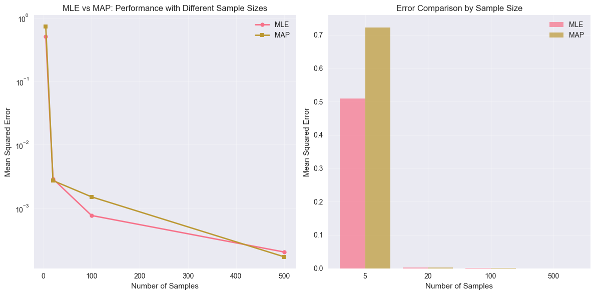
When to use which estimation method:
- Small dataset, strong prior knowledge → MAP
- Small dataset, weak prior knowledge → Full Bayesian (if computational resources allow)
- Large dataset, any prior knowledge → MLE or MAP (similar results)
- Need point estimates quickly → MAP
- Need uncertainty quantification → Full Bayesian
- Regularization is important → MAP (Ridge, Lasso)
- Interpretability is key → MAP with appropriate priors
9. Real-World Applications
Let me show you where MAP estimation shines in practice:
9.1 Text Classification with Naive Bayes
python
# Simulate text classification problem
def naive_bayes_example():
    """
    MAP estimation in Naive Bayes classification
    """
    # Simulate word counts for spam/ham classification
    np.random.seed(42)

    # Prior probabilities (what we know before seeing any emails)
    prior_spam = 0.3  # 30% of emails are spam
    prior_ham = 0.7   # 70% of emails are legitimate

    # Likelihoods (how often words appear in spam vs ham)
    word_probs = {
        'free': {'spam': 0.8, 'ham': 0.1},
        'money': {'spam': 0.7, 'ham': 0.05},
        'meeting': {'spam': 0.1, 'ham': 0.6},
        'urgent': {'spam': 0.6, 'ham': 0.2}
    }

    # New email: "urgent free money"
    email_words = ['urgent', 'free', 'money']

    # Calculate MAP classification
    spam_posterior = prior_spam
    ham_posterior = prior_ham

    for word in email_words:
        spam_posterior *= word_probs[word]['spam']
        ham_posterior *= word_probs[word]['ham']

    # Normalize
    total = spam_posterior + ham_posterior
    spam_prob = spam_posterior / total
    ham_prob = ham_posterior / total

    print(f"Email words: {email_words}")
    print(f"P(Spam|email) = {spam_prob:.3f}")
    print(f"P(Ham|email) = {ham_prob:.3f}")
    print(f"MAP classification: {'SPAM' if spam_prob > ham_prob else 'HAM'}")

naive_bayes_example()
python
Email words: ['urgent', 'free', 'money']
P(Spam|email) = 0.993
P(Ham|email) = 0.007
MAP classification: SPAM
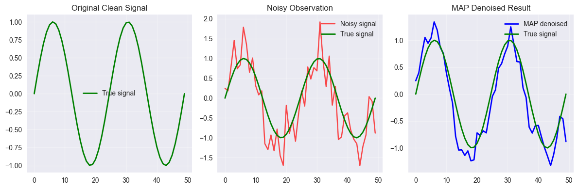
9.2 Image Denoising
python
# Simulate MAP estimation for image denoising
def image_denoising_demo():
    """
    Simplified example of MAP estimation in image denoising
    """
    np.random.seed(42)

    # Create a simple "image" (1D signal for simplicity)
    true_signal = np.sin(np.linspace(0, 4*np.pi, 50))
    noise = 0.5 * np.random.randn(50)
    noisy_signal = true_signal + noise

    # MAP estimation with smoothness prior
    # We believe neighboring pixels should have similar values

    def map_denoise(noisy_data, smoothness_weight=1.0):
        """Simple MAP denoising with smoothness prior"""
        n = len(noisy_data)
        result = noisy_data.copy()

        # Iterative approach (simplified)
        for _ in range(10):
            new_result = result.copy()
            for i in range(1, n-1):
                # Data term: stay close to observations
                data_term = noisy_data[i]

                # Prior term: stay close to neighbors (smoothness)
                smoothness_term = (result[i-1] + result[i+1]) / 2

                # Combine with weights
                new_result[i] = (data_term + smoothness_weight * smoothness_term) / (1 + smoothness_weight)

            result = new_result

        return result

    # Apply MAP denoising
    denoised = map_denoise(noisy_signal, smoothness_weight=2.0)

    # Plot results
    plt.figure(figsize=(12, 4))

    plt.subplot(1, 3, 1)
    plt.plot(true_signal, 'g-', label='True signal', linewidth=2)
    plt.title('Original Clean Signal')
    plt.legend()
    plt.grid(True, alpha=0.3)

    plt.subplot(1, 3, 2)
    plt.plot(noisy_signal, 'r-', alpha=0.7, label='Noisy signal')
    plt.plot(true_signal, 'g-', label='True signal', linewidth=2)
    plt.title('Noisy Observation')
    plt.legend()
    plt.grid(True, alpha=0.3)

    plt.subplot(1, 3, 3)
    plt.plot(denoised, 'b-', label='MAP denoised', linewidth=2)
    plt.plot(true_signal, 'g-', label='True signal', linewidth=2)
    plt.title('MAP Denoised Result')
    plt.legend()
    plt.grid(True, alpha=0.3)

    plt.tight_layout()
    plt.show()

    # Calculate improvement
    noisy_error = np.mean((noisy_signal - true_signal)**2)
    denoised_error = np.mean((denoised - true_signal)**2)

    print(f"Noisy signal error: {noisy_error:.4f}")
    print(f"MAP denoised error: {denoised_error:.4f}")
    print(f"Improvement: {((noisy_error - denoised_error) / noisy_error) * 100:.1f}%")

image_denoising_demo()
python
Noisy signal error: 0.2263
MAP denoised error: 0.0796
Improvement: 64.8%
Free Course
Master Core Python — Your First Step into AI/ML
Build a strong Python foundation with hands-on exercises designed for aspiring Data Scientists and AI/ML Engineers.
Start Free Course →Trusted by 50,000+ learners
Related Course
Master Statistics — Hands-On
Join 5,000+ students at edu.machinelearningplus.com
Explore Course

