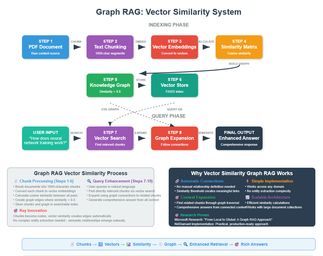
GraphRAG Explained: Your Complete Guide to Knowledge Graph-Powered RAG

Graph RAG is an advanced RAG technique that connects text chunks using vector similarity to build knowledge graphs, enabling more comprehensive and contextual answers than traditional RAG systems. Graph RAG understands connections between chunks and can traverse relationships to provide richer, more complete responses.

Think about the last time you asked an AI a complex question that required connecting multiple pieces of information.

Traditional RAG might find relevant chunks, but tend to miss critical connected information to generate a wholistic answer for the user query.

Graph RAG solves this by understanding relationships between chunks of information in your documents. Instead of just finding similar text, it maps out how everything connects by first building a knowledge graph.

If you’ve ever felt frustrated when AI gives you partial answers because it can’t connect the dots between related information, Graph RAG will change that for you.

1. The Problem We’re Solving

Let me paint you a picture. You have a collection of AI research documents and you ask: “How do the key researchers in deep learning influence each other’s work?”

Traditional RAG takes your question and finds text chunks that mention “deep learning” or “researchers.” You might get separate chunks about Geoffrey Hinton, Yann LeCun, and Yoshua Bengio. But you won’t get the full story of how their collaborations and competing ideas shaped the field.

Graph RAG bridges this gap by first connecting related chunks based on their semantic similarity, then using these connections to find comprehensive information that spans multiple related chunks.

2. How Graph RAG Works

When you ask complex questions that require understanding relationships between multiple concepts, you need more than just individual document chunks – you need to see how everything connects.

The Microsoft Research team tackled this in their 2024 paper “From Local to Global: A Graph RAG Approach to Query-Focused Summarization” by Darren Edge, Ha Trinh, Newman Cheng, Joshua Bradley, Alex Chao, Apurva Mody, Steven Truitt, and Jonathan Larson. Their breakthrough was creating knowledge graphs that capture entity relationships and use community detection to identify related concept clusters.

Graph RAG works by splitting documents into chunks, converting them to vector embeddings, then connecting semantically similar chunks above a certain threshold. This creates a mind map of your entire document collection.

The result is a system that can synthesize information across multiple documents and understand relationships between entities, making it perfect for complex queries that require connecting dots across your knowledge base.

3. Setting Up Your Environment

Before we dive into the code, let’s get everything set up. I’ll assume you have Python and VS Code ready to go.

First, let’s install the packages we need:

conda create -n rag python==3.12
conda activate rag
pip install ipykernel
pip install langchain openai networkx matplotlib pandas numpy
pip install python-dotenv tiktoken pypdf scikit-learn
pip install langchain-community faiss-cpu

Now let’s import everything:

import os
import numpy as np
import pandas as pd
import networkx as nx
import matplotlib.pyplot as plt
from sklearn.metrics.pairwise import cosine_similarity
from dotenv import load_dotenv

# LangChain imports
from langchain_openai import ChatOpenAI, OpenAIEmbeddings
from langchain.text_splitter import RecursiveCharacterTextSplitter
from langchain_community.document_loaders import PyPDFLoader
from langchain_community.vectorstores import FAISS
from langchain.prompts import PromptTemplate

# Load environment variables
load_dotenv()
os.environ["OPENAI_API_KEY"] = os.getenv('OPENAI_API_KEY')

print("All packages imported successfully!")

All packages imported successfully!

Make sure you have a .env file with your OpenAI API key:

OPENAI_API_KEY=your_api_key_here

4. Document Processing and PDF Extraction

Before we can build graphs, we need to extract text from PDF documents and then identify entities and relationships. Let’s start with a simple PDF extraction approach.

You can download the pdf here

# Set the path to our document
document_path = "Artificial Intelligence.pdf"  # Use the path to your PDF

# Load the PDF document
pdf_loader = PyPDFLoader(document_path)
raw_documents = pdf_loader.load()

print(f"Loaded {len(raw_documents)} pages from the PDF")
print(f"First page preview: {raw_documents[0].page_content[:300]}...")

Loaded 14 pages from the PDF
First page preview: Artificial Intelligence and Machine Learning: Fundamentals,
Applications, and Future Directions
Introduction to Artificial Intelligence
Artificial Intelligence represents one of the most transformative technological developments of the
modern era. Defined as the simulation of human intelligence proc...

The PyPDFLoader reads each page as a separate document. This gives us a list of document objects, each containing the text content of one page.

Next, we need to split our documents into chunks. For Graph RAG, we want chunks that are large enough to contain meaningful concepts but small enough to represent focused topics.

# Configure text splitter for Graph RAG
chunk_size = 1000  # Balanced size for meaningful content
chunk_overlap = 200  # Overlap to preserve context

text_splitter = RecursiveCharacterTextSplitter(
    chunk_size=chunk_size,
    chunk_overlap=chunk_overlap,
    separators=["\n\n", "\n", ".", " "]
)

# Split documents into chunks
document_chunks = text_splitter.split_documents(raw_documents)

print(f"Split {len(raw_documents)} pages into {len(document_chunks)} chunks")
print(f"Average chunk size: {sum(len(chunk.page_content) for chunk in document_chunks) // len(document_chunks)} characters")

Split 14 pages into 57 chunks
Average chunk size: 882 characters

We use 1000-character chunks because this gives us chunks that typically contain complete ideas or concepts. The overlap ensures we don’t lose important connections that might span chunk boundaries.

5. Creating Vector Embeddings

Now comes the key part – converting each text chunk into a vector representation that captures its semantic meaning.

These vectors will let us measure how similar chunks are to each other.

# Initialize the embedding model
embedding_model = OpenAIEmbeddings()

print("Embedding model initialized successfully!")

# Create embeddings for all chunks
print("Creating embeddings for all chunks...")
chunk_texts = [chunk.page_content for chunk in document_chunks]

# Get embeddings in batches to avoid rate limits
batch_size = 100
all_embeddings = []

for i in range(0, len(chunk_texts), batch_size):
    batch = chunk_texts[i:i + batch_size]
    batch_embeddings = embedding_model.embed_documents(batch)
    all_embeddings.extend(batch_embeddings)

    if i % 200 == 0:  # Progress indicator
        print(f"Processed {min(i + batch_size, len(chunk_texts))}/{len(chunk_texts)} chunks")

print(f"Created {len(all_embeddings)} embeddings")
print(f"Each embedding has {len(all_embeddings[0])} dimensions")

Embedding model initialized successfully!
Creating embeddings for all chunks...
Processed 57/57 chunks
Created 57 embeddings
Each embedding has 1536 dimensions

Each chunk is now represented as a vector with 1536 dimensions (OpenAI’s embedding size).

These vectors capture the semantic meaning of the text – chunks about similar topics will have similar vectors.

6. Building the Similarity Graph

Now we’ll build our knowledge graph by connecting chunks that are semantically similar. That is we will be using vector similarity to determine relationships.

# Convert embeddings to numpy array for easier computation
embeddings_array = np.array(all_embeddings)

# Calculate cosine similarity between all pairs of chunks
print("Calculating similarity matrix...")
similarity_matrix = cosine_similarity(embeddings_array)

print(f"Similarity matrix shape: {similarity_matrix.shape}")
print(f"Similarity values range from {similarity_matrix.min():.3f} to {similarity_matrix.max():.3f}")

Calculating similarity matrix...
Similarity matrix shape: (57, 57)
Similarity values range from 0.713 to 1.000

The similarity matrix tells us how similar every chunk is to every other chunk. Values close to 1 mean very similar, values close to 0 mean very different.

Now let’s build the graph by connecting chunks that are similar enough

# Set similarity threshold for creating edges
similarity_threshold = 0.8  # Only connect chunks that are highly similar

# Create the knowledge graph
G = nx.Graph()

# Add nodes (one for each chunk)
for i, chunk in enumerate(document_chunks):
    G.add_node(i, 
               content=chunk.page_content,
               page=chunk.metadata.get('page', 0),
               length=len(chunk.page_content))

print(f"Added {G.number_of_nodes()} nodes to the graph")

Added 57 nodes to the graph

Each chunk becomes a node in our graph, with the chunk content and metadata stored as node attributes.

# Add edges based on similarity threshold
edge_count = 0
total_pairs = len(document_chunks) * (len(document_chunks) - 1) // 2

print("Creating edges based on similarity...")

for i in range(len(document_chunks)):
    for j in range(i + 1, len(document_chunks)):
        similarity = similarity_matrix[i][j]

        # Create edge if similarity is above threshold
        if similarity >= similarity_threshold:
            G.add_edge(i, j, weight=similarity)
            edge_count += 1

print(f"Created {edge_count} edges from {total_pairs} possible pairs")
print(f"Graph density: {nx.density(G):.3f}")
print(f"Average similarity of connected chunks: {np.mean([data['weight'] for _, _, data in G.edges(data=True)]):.3f}")

Creating edges based on similarity...
Created 1017 edges from 1596 possible pairs
Graph density: 0.637
Average similarity of connected chunks: 0.838

We only create edges between chunks that have similarity above our threshold (0.8). This ensures we only connect chunks that are truly related, creating a meaningful knowledge graph.

7. Analyzing the Knowledge Graph

Let’s analyze our knowledge graph to understand the structure of knowledge in our documents.

# Basic graph statistics
print(" GRAPH ANALYSIS:")
print("=" * 40)
print(f"Total nodes (chunks): {G.number_of_nodes()}")
print(f"Total edges (connections): {G.number_of_edges()}")
print(f"Graph density: {nx.density(G):.3f}")
print(f"Number of connected components: {nx.number_connected_components(G)}")

# Find most connected chunks
node_degrees = dict(G.degree())
top_connected = sorted(node_degrees.items(), key=lambda x: x[1], reverse=True)[:5]

print("\n Most Connected Chunks:")
for node_id, degree in top_connected:
    chunk_preview = document_chunks[node_id].page_content[:100].replace('\n', ' ')
    print(f"Node {node_id} ({degree} connections): {chunk_preview}...")

 GRAPH ANALYSIS:
========================================
Total nodes (chunks): 57
Total edges (connections): 1017
Graph density: 0.637
Number of connected components: 1

 Most Connected Chunks:
Node 51 (54 connections): and John McCarthy to the current era of large language models and autonomous systems, AI has demonst...
Node 2 (53 connections): expectations and limitations in computational power. However, the field experienced a renaissance in...
Node 3 (51 connections): processing, and autonomous systems. Foundations of Machine Learning Machine Learning, a subset of ar...
Node 11 (51 connections): widespread interest and investment in deep learning technologies. Subsequent developments have conti...
Node 16 (51 connections): team, and RoBERTa by Yinhan Liu and colleagues at Facebook AI Research, have demonstrated the effect...

The most connected chunks are often the most important concepts in your document collection – they appear in contexts similar to many other chunks.

# Find communities of related chunks
print("\n Finding communities of related chunks...")
communities = list(nx.community.greedy_modularity_communities(G))

print(f"Found {len(communities)} communities:")
for i, community in enumerate(communities[:3]):  # Show first 3 communities
    if len(community) > 1:
        print(f"\nCommunity {i+1} ({len(community)} chunks):")
        for node_id in list(community)[:3]:  # Show first 3 members
            chunk_preview = document_chunks[node_id].page_content[:80].replace('\n', ' ')
            print(f"  - Chunk {node_id}: {chunk_preview}...")

 Finding communities of related chunks...
Found 2 communities:

Community 1 (30 chunks):
  - Chunk 0: Artificial Intelligence and Machine Learning: Fundamentals, Applications, and Fu...
  - Chunk 1: who proposed the famous Turing Test in 1950 as a criterion for machine intellige...
  - Chunk 2: expectations and limitations in computational power. However, the field experien...

Community 2 (27 chunks):
  - Chunk 27: functions. The REINFORCE algorithm, developed by Ronald Williams, was one of the...
  - Chunk 28: vast amounts of medical data, identify complex patterns that may not be apparent...
  - Chunk 29: screening for breast cancer, chest X-ray analysis for pneumonia detection, and C...

Community detection reveals clusters of highly interconnected chunks. These often represent different topics or themes in your document collection.

8. Visualizing the Knowledge Graph

Let’s visualize our knowledge graph to see how chunks connect to each other.

# Create a visualization of the graph
plt.figure(figsize=(15, 10))

# Use only a subset for visualization if graph is too large
if G.number_of_nodes() > 50:
    # Get the largest connected component for visualization
    largest_cc = max(nx.connected_components(G), key=len)
    G_vis = G.subgraph(largest_cc).copy()
    print(f"Visualizing largest connected component with {G_vis.number_of_nodes()} nodes")
else:
    G_vis = G

# Calculate node sizes based on degree (number of connections)
node_sizes = [G_vis.degree(node) * 50 + 100 for node in G_vis.nodes()]

# Color nodes by their community
try:
    communities_vis = list(nx.community.greedy_modularity_communities(G_vis))
    node_colors = []
    colors = ['lightblue', 'lightgreen', 'orange', 'pink', 'yellow', 'lightcoral']

    for node in G_vis.nodes():
        for i, community in enumerate(communities_vis):
            if node in community:
                node_colors.append(colors[i % len(colors)])
                break
        else:
            node_colors.append('gray')
except:
    node_colors = ['lightblue'] * G_vis.number_of_nodes()

# Create layout
pos = nx.spring_layout(G_vis, k=3, iterations=50)

# Draw the graph
nx.draw(G_vis, pos,
        node_color=node_colors,
        node_size=node_sizes,
        with_labels=True,
        font_size=8,
        font_weight='bold',
        edge_color='gray',
        alpha=0.7,
        width=0.5)

plt.title("Knowledge Graph - Document Chunks Connected by Similarity", fontsize=16)
plt.axis('off')
plt.show()

Visualizing largest connected component with 57 nodes

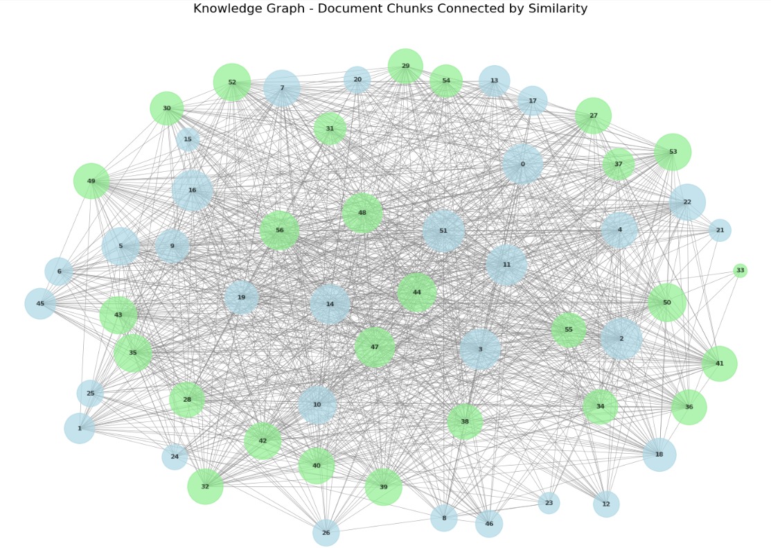
This visualization shows how chunks in your documents connect to each other.

Larger nodes have more connections, indicating they’re central to multiple topics. Different colors represent different communities of related chunks.

9. Graph-Enhanced Retrieval

Now let’s start using our knowledge graph to enhance retrieval!

When someone asks a question, we’ll use the graph to find not just directly relevant chunks, but also related chunks through graph traversal.

First, let’s create a traditional vector store for comparison

# Create traditional vector store using embeddings
vector_store = FAISS.from_documents(document_chunks, embedding_model)

print("Vector store created successfully!")

Vector store created successfully!

This creates a traditional RAG system that we can compare against our Graph RAG approach.

Now let’s build the graph-enhanced retrieval system

def graph_enhanced_retrieval(query, vector_store, graph, embeddings_array, k=5, expansion_factor=2):
    """
    Retrieve documents using both vector similarity and graph relationships

    Args:
        query: User's question
        vector_store: Traditional FAISS vector store
        graph: Our knowledge graph
        embeddings_array: Array of chunk embeddings
        k: Number of initial chunks to retrieve
        expansion_factor: How many connected chunks to add per initial chunk

    Returns:
        enhanced_chunks: List of chunks with both direct and graph-connected results
    """

    print(f" Processing query: {query}")

    # Step 1: Traditional vector search to get initial relevant chunks
    initial_results = vector_store.similarity_search_with_score(query, k=k)
    initial_chunk_ids = []

    # Find the chunk IDs for the initial results
    for doc, score in initial_results:
        for i, chunk in enumerate(document_chunks):
            if chunk.page_content == doc.page_content:
                initial_chunk_ids.append(i)
                break

    print(f" Found {len(initial_chunk_ids)} initial relevant chunks")

    # Step 2: Expand using graph connections
    expanded_chunk_ids = set(initial_chunk_ids)

    for chunk_id in initial_chunk_ids:
        if chunk_id in graph:
            # Get connected chunks sorted by similarity weight
            neighbors = list(graph.neighbors(chunk_id))
            neighbor_weights = [(n, graph[chunk_id][n]['weight']) for n in neighbors]
            neighbor_weights.sort(key=lambda x: x[1], reverse=True)

            # Add top connected chunks
            for neighbor_id, weight in neighbor_weights[:expansion_factor]:
                expanded_chunk_ids.add(neighbor_id)

    print(f" Expanded to {len(expanded_chunk_ids)} chunks using graph connections")

    # Step 3: Rank all chunks by similarity to query
    query_embedding = embedding_model.embed_query(query)
    chunk_scores = []

    for chunk_id in expanded_chunk_ids:
        chunk_embedding = embeddings_array[chunk_id]
        similarity = cosine_similarity([query_embedding], [chunk_embedding])[0][0]
        chunk_scores.append((chunk_id, similarity, chunk_id in initial_chunk_ids))

    # Sort by similarity score
    chunk_scores.sort(key=lambda x: x[1], reverse=True)

    # Return top chunks with metadata
    enhanced_chunks = []
    for chunk_id, score, is_initial in chunk_scores[:k*2]:  # Return more chunks
        enhanced_chunks.append({
            'chunk': document_chunks[chunk_id],
            'similarity': score,
            'source': 'direct' if is_initial else 'graph',
            'chunk_id': chunk_id
        })

    return enhanced_chunks

# Test graph-enhanced retrieval
test_query = "How do neural networks learn from data?"
enhanced_results = graph_enhanced_retrieval(test_query, vector_store, G, embeddings_array)

print(f"\n Retrieved {len(enhanced_results)} chunks:")
for i, result in enumerate(enhanced_results[:5]):
    source_type = result['source']
    similarity = result['similarity']
    content_preview = result['chunk'].page_content[:150].replace('\n', ' ')
    print(f"\n{i+1}. [{source_type.upper()}] (similarity: {similarity:.3f})")
    print(f"   {content_preview}...")

 Processing query: How do neural networks learn from data?
 Found 5 initial relevant chunks
 Expanded to 11 chunks using graph connections

 Retrieved 10 chunks:

1. [DIRECT] (similarity: 0.833)
   The theoretical foundations of machine learning draw heavily from statistics, probability theory, and optimization. The concept of learning from data ...

2. [DIRECT] (similarity: 0.820)
   learning algorithm for neural networks. However, the limitations of single-layer perceptrons, famously highlighted by Marvin Minsky and Seymour Papert...

3. [DIRECT] (similarity: 0.819)
   law of effect states that behaviors followed by satisfying consequences are more likely to be repeated. Richard Sutton and Andrew Barto formalized man...

4. [DIRECT] (similarity: 0.816)
   The conceptual foundation of neural networks dates back to the 1940s with the work of Warren McCulloch and Walter Pitts, who created the first mathema...

5. [DIRECT] (similarity: 0.814)
   for image classification tasks. The development of the bag-of-words model for computer vision, inspired by techniques from natural language processing...

This retrieval system first finds directly relevant chunks, then expands the search using graph connections to find related information that might not be directly similar to the query but is connected to relevant chunks.

10. Comparing Graph RAG vs Traditional RAG

Let’s see the difference between Graph RAG and traditional RAG side by side

def compare_retrieval_methods(query, vector_store, graph, embeddings_array):
    """Compare traditional RAG vs Graph RAG"""

    print(" TRADITIONAL RAG:")
    print("=" * 50)
    traditional_results = vector_store.similarity_search_with_score(query, k=3)

    for i, (doc, score) in enumerate(traditional_results):
        content = doc.page_content[:150].replace('\n', ' ')
        print(f"Result {i+1} (score: {score:.3f}):")
        print(f"{content}...")
        print("-" * 30)

    print("\n GRAPH RAG:")
    print("=" * 50)
    graph_results = graph_enhanced_retrieval(query, vector_store, graph, embeddings_array, k=3)

    for i, result in enumerate(graph_results[:5]):
        source_type = result['source']
        similarity = result['similarity']
        content_preview = result['chunk'].page_content[:150].replace('\n', ' ')
        print(f"Result {i+1} [{source_type.upper()}] (similarity: {similarity:.3f}):")
        print(f"{content_preview}...")
        print("-" * 30)

# Compare both methods
comparison_query = "What are the applications of deep learning in computer vision?"
compare_retrieval_methods(comparison_query, vector_store, G, embeddings_array)

 TRADITIONAL RAG:
==================================================
Result 1 (score: 0.256):
for image classification tasks. The development of the bag-of-words model for computer vision, inspired by techniques from natural language processing...
------------------------------
Result 2 (score: 0.291):
fully connected layers for image classification. The hierarchical feature learning capability of CNNs mimics the structure of the visual cortex, makin...
------------------------------
Result 3 (score: 0.293):
team, and RoBERTa by Yinhan Liu and colleagues at Facebook AI Research, have demonstrated the effectiveness of transfer learning in NLP. The emergence...
------------------------------

GRAPH RAG:
==================================================
 Processing query: What are the applications of deep learning in computer vision?
 Found 3 initial relevant chunks
 Expanded to 7 chunks using graph connections
Result 1 [DIRECT] (similarity: 0.872):
for image classification tasks. The development of the bag-of-words model for computer vision, inspired by techniques from natural language processing...
------------------------------
Result 2 [DIRECT] (similarity: 0.855):
fully connected layers for image classification. The hierarchical feature learning capability of CNNs mimics the structure of the visual cortex, makin...
------------------------------
Result 3 [DIRECT] (similarity: 0.854):
team, and RoBERTa by Yinhan Liu and colleagues at Facebook AI Research, have demonstrated the effectiveness of transfer learning in NLP. The emergence...
------------------------------
Result 4 [GRAPH] (similarity: 0.848):
development of modern deep learning techniques. His work on restricted Boltzmann machines, deep belief networks, and more recently, capsule networks, ...
------------------------------
Result 5 [GRAPH] (similarity: 0.818):
widespread interest and investment in deep learning technologies. Subsequent developments have continued to push the boundaries of deep learning. The ...
------------------------------

You’ll notice that Graph RAG retrieves more contextually relevant documents because it understands the relationships between concepts.

11. Building a Complete Graph RAG Answer System

Let’s put everything together into a complete question-answering system that uses our knowledge graph

def answer_with_graph_rag(question, vector_store, graph, embeddings_array, llm):
    """Complete Graph RAG answering system"""

    print(f" Question: {question}")
    print("\n Searching with Graph RAG...")

    # Get enhanced retrieval results
    enhanced_results = graph_enhanced_retrieval(
        question, vector_store, graph, embeddings_array, k=3, expansion_factor=2
    )

    # Show what chunks were used
    direct_chunks = [r for r in enhanced_results if r['source'] == 'direct']
    graph_chunks = [r for r in enhanced_results if r['source'] == 'graph']

    print(f" Using {len(direct_chunks)} directly relevant chunks")
    print(f" Using {len(graph_chunks)} graph-connected chunks")

    # Combine context from retrieved chunks
    contexts = []
    for result in enhanced_results[:8]:  # Use top 8 chunks
        contexts.append(result['chunk'].page_content)

    combined_context = "\n\n".join(contexts)

    # Create answer using retrieved context
    answer_prompt = PromptTemplate(
        input_variables=["question", "context"],
        template="""Based on the following context from connected document chunks, provide a comprehensive answer to the question.

Context:
{context}

Question: {question}

Provide a detailed answer that leverages the relationships between the connected chunks:"""
    )

    # Generate answer
    chain = answer_prompt | llm
    response = chain.invoke({
        "question": question,
        "context": combined_context[:4000]  # Limit context length
    })

    print("\n Answer:")
    print("=" * 50)
    print(response.content)

    return response.content

# Initialize LLM for answer generation
llm = ChatOpenAI(
    temperature=0,
    model_name="gpt-4o-mini",
    max_tokens=1000
)

# Test the complete system
user_question = "How has deep learning evolved from early neural networks?"
answer = answer_with_graph_rag(user_question, vector_store, G, embeddings_array, llm)

 Question: How has deep learning evolved from early neural networks?

 Searching with Graph RAG...
 Processing query: How has deep learning evolved from early neural networks?
 Found 3 initial relevant chunks
 Expanded to 5 chunks using graph connections
 Using 3 directly relevant chunks
 Using 2 graph-connected chunks

 Answer:
==================================================
Deep learning has undergone a significant evolution from its early neural network roots, marked by several key developments and breakthroughs that have transformed the field.

1. **Foundational Concepts**: The conceptual foundation of neural networks can be traced back to the 1940s with the pioneering work of Warren McCulloch and Walter Pitts, who created the first mathematical model of an artificial neuron. However, the initial enthusiasm for neural networks waned due to the limitations of single-layer perceptrons, as highlighted by Marvin Minsky and Seymour Papert in their 1969 book "Perceptrons." This critique led to a decline in research and interest in neural networks for several years.

2. **Revival through Backpropagation**: The revival of interest in neural networks began in the 1980s with the introduction of the backpropagation algorithm. This algorithm, independently discovered by researchers including Paul Werbos, David Rumelhart, Geoffrey Hinton, and Ronald Williams, allowed for the efficient training of multi-layer neural networks. By enabling the computation of gradients, backpropagation made it feasible to learn complex non-linear mappings from inputs to outputs, thus laying the groundwork for deeper architectures.

3. **Advancements in Architectures**: The evolution of deep learning saw the development of various architectures that significantly improved performance in specific tasks. For instance, Yann LeCun's work on Convolutional Neural Networks (CNNs) in the 1980s, particularly the LeNet architecture, demonstrated the effectiveness of combining convolutional layers with pooling and fully connected layers for image classification. This hierarchical feature learning capability mimics the structure of the visual cortex, making CNNs particularly well-suited for visual tasks.

4. **Breakthroughs in Computer Vision**: The deep learning revolution gained substantial momentum with the introduction of AlexNet in 2012, designed by Alex Krizhevsky, Ilya Sutskever, and Geoffrey Hinton. AlexNet achieved a dramatic improvement in image classification accuracy during the ImageNet Large Scale Visual Recognition Challenge, showcasing the power of deep convolutional networks and GPU computing. This success not only validated deep learning techniques but also sparked widespread interest and investment in the field.

5. **Continued Innovation**: Following AlexNet, subsequent architectures such as VGGNet and ResNet further pushed the boundaries of performance in computer vision. VGGNet, developed by Karen Simonyan and Andrew Zisserman, demonstrated the effectiveness of very deep networks with small convolutional filters, while ResNet introduced the concept of residual learning, allowing for the training of extremely deep networks without suffering from degradation.

6. **Broader Applications**: Beyond computer vision, deep learning has expanded into other domains, including natural language processing (NLP). Yoshua Bengio's contributions to recurrent neural networks and attention mechanisms have been crucial for NLP applications, showcasing the versatility and adaptability of deep learning techniques across various fields.

7. **Emerging Techniques**: The evolution of deep learning continues with the exploration of new architectures and techniques, such as restricted Boltzmann machines, deep belief networks, and capsule networks, which Geoffrey Hinton has been instrumental in developing. These innovations aim to further enhance the capabilities of neural networks and address existing limitations.

In summary, deep learning has evolved from simple neural network models to complex architectures capable of achieving state-of-the-art performance in various applications. This evolution has been driven by foundational advancements in algorithms, innovative architectures, and breakthroughs in specific domains, particularly computer vision and natural language processing. The field continues to grow, with ongoing research pushing the boundaries of what neural networks can achieve.

This system gives you comprehensive answers that consider not just direct matches, but also related concepts and their relationships.

While Graph RAG requires more computational resources and setup complexity compared to traditional RAG, the improvement in answer quality makes it worthwhile for applications where comprehensive understanding is crucial.