
Chi-Square test – How to test statistical significance for categorical data?
Chi-square test is used to determine whether there is a statistically significant difference between the observed frequency and the expected frequency in one or more categories of the contingency table
What is chi-square test and its purpose?
Chi-square test was invented in the year ‘1900’ by the revered mathematician ‘Karl Pearson’. Chi-square test, also written as χ2 test is used to determine whether there is a statistically significant difference between the observed frequency and the expected frequency in one or more categories of the contingency table. Where, a contingency table is a type of table in a matrix form that displays the frequency distribution of the variables.
Where is chi-square test used
Chi-square test is used in the following situations:
- When needed to estimate how closely an observed frequency matches expected frequency.
- To estimate whether two categorical variables are independent.
- Used when you have to find statistically significant difference between categorical data.
Example for chi-square test
Let’s see where Chi-square test can be used to see if there is a difference in expected vs observed frequencies in a categorical variable. In this case only one categorical variable is involved.
python
import pandas as pd
no_of_customers = 100
Observed_Data = {'Red' : [20],
                 'Green' : [19],
                 'Blue' : [21],
                 'Black' : [9],
                 'White' : [31]
                 }
Expected_Data = {'Red' : [20],
                 'Green' : [20],
                 'Blue' : [20],
                 'Black' : [20],
                 'White' : [20]
                 }
observed_df = pd.DataFrame(Observed_Data, columns = ['Red', 'Green', 'Blue', 'Black', 'White'])
expected_df = pd.DataFrame(Expected_Data, columns = ['Red', 'Green', 'Blue', 'Black', 'White'])
print('Observed Data:n',observed_df)
print("")
print('Expected Data:n',expected_df)
python
Observed Data:
    Red  Green  Blue  Black  White
0   20     19    21      9     31

Expected Data:
    Red  Green  Blue  Black  White
0   20     20    20     20     20
Consider that there are 100 people going to a car dealership. If everything is normal, you might expect that people’s preferences on the car color will be equally distributed. But looking at the observed data you can say that people prefer the color ‘white’ more than the other colors. This conclusion/fact is what chi-square test can prove.
Now lets look back into the original problem in hand i.e. Malware Detection. Consider there are two types of ‘os’ tabulated against whether the particular ‘os’ is infected or not.
Malware Detection
python
Data = {'OS Type' : ['os1', 'os2', 'os1', 'os1', 'os2', 'os2', '.....'],
        'Infected/ Not Infected' : [1, 0, 0, 1, 1, 0, '.....']
       }
# where 1 represents infected and 0 represents not infected.
malware_data = pd.DataFrame(Data, columns = ['OS Type', 'Infected/ Not Infected'])
malware_data
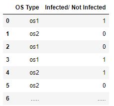
Let’s assume that the dataset is extending over 100 entries.
Contingency Table
The contingency table consists of the frequency distribution of the variables. The contingency table for the above dataset will be:
python
contingency_table = {'Infected' : [40, 10],
                     'Not Infected' : [30, 40]}
df_contingency_table = pd.DataFrame(contingency_table, index = ['OS1', 'OS2'])
df_contingency_table
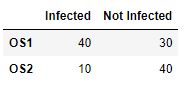
The above values are totally random and it is just created for computation sake. These values say that there is a total of 120 observations. Just by looking at the table, you can say that OS1 is more vulnerable to malware than OS2. Now let’s apply chi-square test.
How to perform chi-square test
Steps involved in χ2 test
Step 1: Formulate the null hypothesis and the alternate hypothesis. It looks as follows:
H0 = The Observed frequency and the expected frequency are the same.
H1 = At least one of the observed frequency is not as same as the expected frequency.
In general, significance level taken is:
α = 0.05 which is 5%
Step 2: To Compute the expected frequency.
If you have only one categorical variable:
Suppose you number of values(n) to be 100 and number of categories(q) to be 5.
Expected_frequency = 100 / 5 = 20
Whereas if you have two categorical variables the calculation is slightly different. It will be as follows:
where,
N = a + b + c + d
Now you have the observed frequency and the expected frequency, let’s calculate the chi-square statistic. Therefore, the observed and expected values are:
python
observed = {'Infected' : [40, 10],
            'Not Infected' : [30, 40]}
df_observed = pd.DataFrame(contingency_table, index = ['OS1', 'OS2'])

expected = {'Infected' : [29.16, 20.83],
            'Not Infected' : [40.83, 29.11]}
df_expected = pd.DataFrame(expected, index = ['OS1', 'OS2'])

print('Observed values:')
print(df_observed)
print("")
print('Expected values:')
print(df_expected)
python
Observed values:
     Infected  Not Infected
OS1        40            30
OS2        10            40

Expected values:
     Infected  Not Infected
OS1     29.16         40.83
OS2     20.83         29.11
Formula for chi-square statistic
The formula for chi-square test is:

The formula is simple. You find the sum of the difference between Observed Frequency and Expected Frequency whole divided by Expected Frequency.
Calculation

The third step is to find the degree of freedom
How to calculate Degree of Freedom?
Consider there are 5 types of chocolates and 5 people. Only the first 4 people get to choose their favorite chocolate and the final person has to select the leftover chocolate because that person has no other choice. This is called ‘Degrees of Freedom’. The formula for the degree of freedom is:
d.o.f = (n-1)(m-1)
Where,
n and m correponds to number of unique values in each categorical variables. In our case it would be:
d.o.f = (2-1)(2-1) = 1
Critical value of chi-square statistic
The fourth step would be to find the critical value of chi-square test statistic. To find this value, You need the chi-square table. To access the chi-square table, you can either directly search “chi-square-table” in google or use the following link chi-square table

The rows represent d.o.f (i.e. 1) and the column represents significance value(i.e. 0.05). So, the critical value is 3.841
Now, there are two cases,
Case 1: If the chi-square statistic > critical value, H0 gets Rejected.
Case 2: If the chi-square statistic < critical value, H0 is Accepted.
In our case, 16.559 > 3.841 and therefore the H0 gets Rejected. This leads to the conclusion that at least one of the observed frequency is not equal to expected frequency.
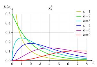
Chi-square distribution
Chi-Square calculation in python when you know the observed and expected values
Now, lets at how the chi-square calculation is done using python. To do the calculation, you will need a library called scipy.
python
import scipy.stats as stats
crit = stats.chi2.ppf(q = 0.95, df = 1)
print("Critical value=",crit)

stats.chisquare(f_obs = df_observed, f_exp = df_expected)
print('Chi-square statistic=',stats.chisquare(f_obs = df_observed, f_exp = df_expected))
python
Critical value= 3.841458820694124
Chi-square statistic= Power_divergenceResult(statistic=array([9.66045262, 6.94654564]), pvalue=array([0.00188277, 0.00839812]))
This output shows us the critical value and the chi-square statistic calculated. The chi-square statistic is 16.60699826 ( 9.66045262 + 6.94654564). Therefore,
Chi-square statistic (16.606) > Critical Value (3.841) and thus our H0 gets Rejected.
Chi-Square calculation in python when you have a contingency table
The dataset below is called ‘Churn_modelling.csv’. The term ‘churn’ refers to ‘lose of a client or a customer’. The dataset lists various customers details such as their ID, Surname, their country, age, gender, no. of products they bought and so on. The final column ‘Exited’ refers whether the particular customer is still in business with the respective company or not (0 refers to ‘No’ and 1 refers to ‘Yes’).
Consider if you are trying to find whether there is any relationship between a person’s gender and whether they have exited or not.
First step would be to import the libraries and the dataset.
python
import pandas as pdThen the dataset is imported using read_csv() and the first 5 rows are displayed using the head().
python
data = pd.read_csv('https://raw.githubusercontent.com/selva86/datasets/master/Churn_Modelling.csv')

# displays the first 5 rows.
data.head(5)
The next step, would be to compute the contingency table for the columns ‘Gender’ and ‘Exited’. The pandas library has a method called ‘crosstab’ which can be used to compute the contingency table.
python
contingency = pd.crosstab(data.Gender, data.Exited)
contingency
python
Exited	0	1
Gender
Female	3404	1139
Male	4559	898
The scipy library consists of scipy.stats.chi2_contingency which can be used to apply the chi square test to the contingency table.
This function outputs :
1. Chi square statistic,
2. P-Value,
3. Degrees of Freedom,
4. Expected Frequency.
The critical value is also computed using scipy.stats.chi2.ppf()
python
import numpy as np
from scipy.stats import chi2_contingency
import scipy.stats as stats

crit = stats.chi2.ppf(q = 0.95, df = 1)

print("critical value:", crit)

chi_statistic, p_value, dof, expected_freq = chi2_contingency(contingency)

print("chi2 statistic = %.5f" % chi_statistic)

print("p-value = %.5f" % p_value)

print("Degrees of Freedom (D.O.F) = ", dof)

print("Expected Frequencies:")

print(expected_freq)
python
critical value: 3.841458820694124
chi2 statistic = 112.91857
p-value = 0.00000
Degrees of Freedom (D.O.F) =  1
Expected Frequencies:
[[3617.5909  925.4091]
 [4345.4091 1111.5909]]
The chi square statistic obtained is 112.91857 and the critical value obtained is 3.841, Recall,
If Chi-Square statistic > critical value , the H0 gets Rejected. When this happens, the p-value is usually less than the significance level ( <0.05).
Thus our H0 gets Rejected.
Limitations of chi-square test
Here are some of the limitations of chi-square test:
The test is very sensitive to the sample size. That is, as sample size increases, absolute differences becomes smaller and smaller proportion of the expected value. What this means is that a reasonably strong association may not come up as significant if the sample size is small, and conversely, in large samples, you might find statistical significance when the findings are small which means the findings are not substantively significant, although they are statistically significant.
It is difficult to interpret when the numbers of categories are more than 20.
Free Course
Master Core Python — Your First Step into AI/ML
Build a strong Python foundation with hands-on exercises designed for aspiring Data Scientists and AI/ML Engineers.
Start Free Course →Trusted by 50,000+ learners

Related Course
Master Statistics — Hands-On
Join 5,000+ students at edu.machinelearningplus.com
Explore Course
Related Articles